Quick start
Loading the library
To use sajou simply import the library as you would usually do:
import sajou as sj
That’s it! After this, you are ready to start building your model.
Building the model
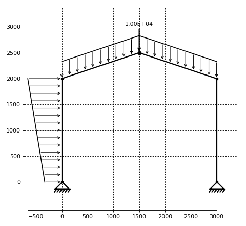
A simple frame structure as described in the figure below will be calculated.
(Source code, png, hires.png, pdf)

Geometry
To build the model a Model has to be created:
# Initialize a Model instance of a 2D model
m = sj.Model(name='Model 1', dimensionality='2D')
The geometry of the problem can then be defined by means of Node, which is conveniently wrapped in the method Model2D.node() of the class Model:
# add nodes
n1 = m.node(0., 0.)
n2 = m.node(0., 2000.)
n3 = m.node(1500., 2500.)
n4 = m.node(3000., 2000.)
n5 = m.node(3000., 0.)
Beam elements (Beam2D) are created using a method of the class model.Model:
# add segment
b1 = m.beam(node1=n1, node2=n2)
b2 = m.beam(node1=n2, node2=n3)
b3 = m.beam(node1=n3, node2=n4)
b4 = m.beam(node1=n4, node2=n5)
Material and cross-section
For this example, the material consist of a timber glulam, with an modulus of elasticity (MOE) equals to 12 GPa. The cross-section of the beam is defined as a rectangular section.
See also
sections.BeamSection to understand how to pass different parameters
| Property | value | units |
|---|---|---|
| MOE | 12 | GPa |
| width | 100 | mm |
| depth | 300 | mm |
The material is defined by means of the Model.material() method, which creates an instance of the class Material.
This is then assigned to a BeamSection instance, using the Model.beam_section() method and giving the
parameter type='rectangular':
# create material
mat = m.material(name='glulam', data=(12e3, ), type='isotropic')

# create beam section
section1 = m.beam_section(name='glulam section', material=mat, data=(
    100, 300), type='rectangular')
The above created BeamSection now needs to be assigned to a Beam2D instance:
# add beam section to the beams
b1.assign_section(section1)
b2.assign_section(section1)
b3.assign_section(section1)
b4.assign_section(section1)
Applying loads and border conditions
Sajou supports the application of both concentrated loads as well as distributed loads. For this, the methods Model.load() and Beam2D.distributed_load() are used.
The border conditions (BCs) are defined with the method Model.bc():
# Add border conditions
m.bc(node=n1, v1=0., v2=0.)
m.bc(node=n5, v1=0., v2=0.)

# Add load
m.load(node=n3, f2=-10e3)

# Distributed load
b1.distributed_load(p1=-1, p2=-2, direction='y', coord_system='local')
b2.distributed_load(p1=-1, direction='y', coord_system='global')
b3.distributed_load(p1=-1, direction='y', coord_system='global')
See also
Concentrated and distributed moments are also supported. See the methods Model.load() and Beam2D.distributed_moment()
End release (adding a hinge)
It is also possible to add hinges at a given node, by means of the Beam2D.release_end() method.
This method adds an additional degree of freedom at the respective node, effectively uncoupling the rotation from the rest of the system:
# release end
b2.release_end(which=2)
Visualizing the model
A visual inspection of the model is crucial to easily spot problems in the model.
To see the current state of the model a Display instance has to be instantiated and a Matplotlib axis has to be passed (this might change in the future):
import matplotlib.pyplot as plt
fig = plt.figure(figsize=(6., 5.5))
ax = fig.add_subplot(111)
disp = sj.Display(theme='dark')
ax = disp.plot_geometry(ax=ax, model=m)
plt.show()
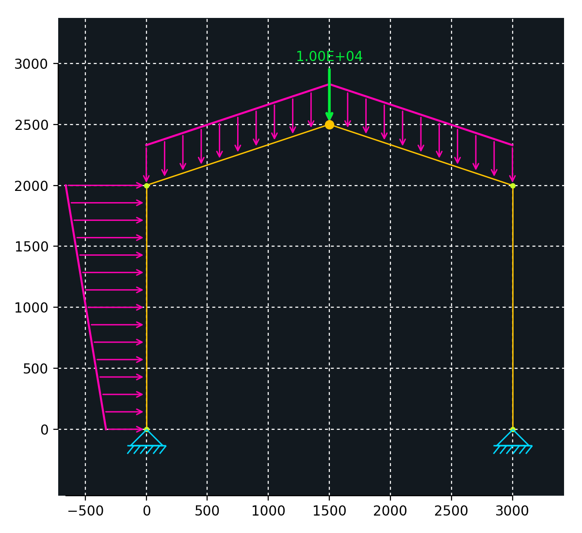
A figure similar to the one shown below should be created.
(Source code, png, hires.png, pdf)

Solving the system
For this example, the implemented static solver (StaticSolver) is used:
from sajou.solvers import StaticSolver
# Define output variables
output = ['nodal displacements', 'internal forces', 'end forces']
# Create the StaticSolver instance
solver = StaticSolver(model=m, output=output)
# Solve the system
res = solver.solve()
After this, a Result object is created (stored as res in the example), which contains the required results of the system.
Postprocessing
The previously obtained Result object is then used in the post-processing of the model.
This is done by means of a Postprocess object, which defines several methods to obtain values
of section forces in a specified element and to plot the results using the above mentioned Display class.
Let us begin by extracting values o the moment, shear and axial force along a specified beam (say beam No. 2):
# Postprocess the results
post = sj.Postprocess(result=res)
# get the values at the center of the beam
m_0 = post.calc_moment_at(pos=0.5, element=b2, unit_length=True)
s_0 = post.calc_shear_at(pos=0.5, element=b2, unit_length=True)
a_0 = post.calc_axial_at(pos=0.5, element=b2, unit_length=True)
As can be seen in the code above, the option unit_length is set to True, which indicates that the values given
for the pos parameter must be in the range [0, 1].
Note
The pos parameter of the calc_moment_at() also accept an array-like argument, so that the
result can be obtained at different points over the beam element at once.
This also holds for the calc_shear_at() and calc_axial_at() methods.
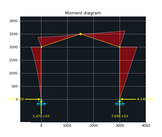
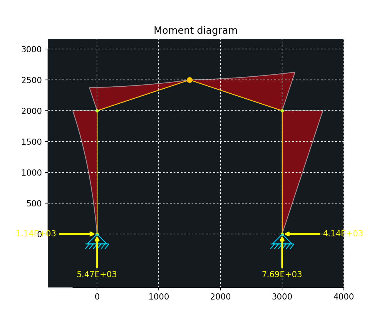
Finally, nice plots can be obtained for the different section forces (moment, shear and axial force):
# create the matplotlib figures
fig1 = plt.figure(figsize=(6.5, 5.5))
fig2 = plt.figure(figsize=(6.5, 5.5))
fig3 = plt.figure(figsize=(6.5, 5.5))
fig4 = plt.figure(figsize=(6.5, 5.5))
ax1 = fig1.add_subplot(111)
ax2 = fig2.add_subplot(111)
ax3 = fig3.add_subplot(111)
ax4 = fig4.add_subplot(111)
# plot the moment along the frame elements
ax1 = disp.plot_internal_forces(ax=ax1, result=res, component='moment')
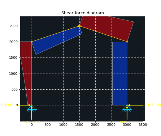
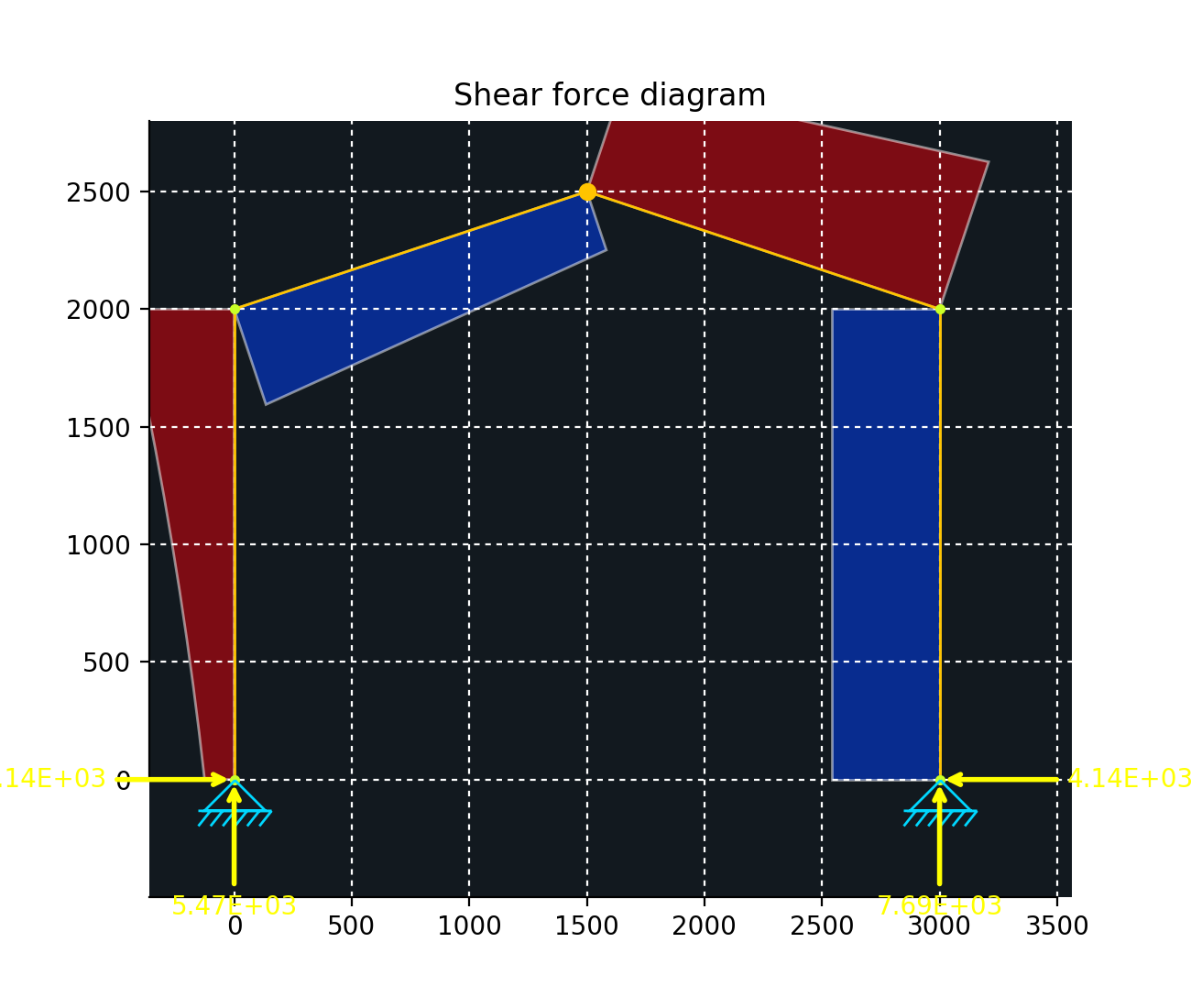
# plot the shear force the frame elements
ax2 = disp.plot_internal_forces(ax=ax2, result=res, component='shear')
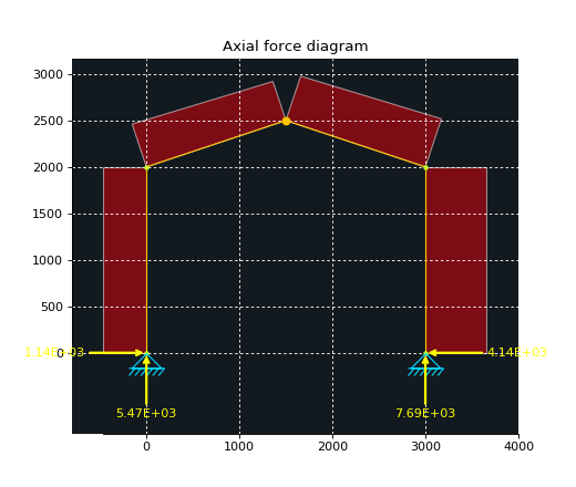
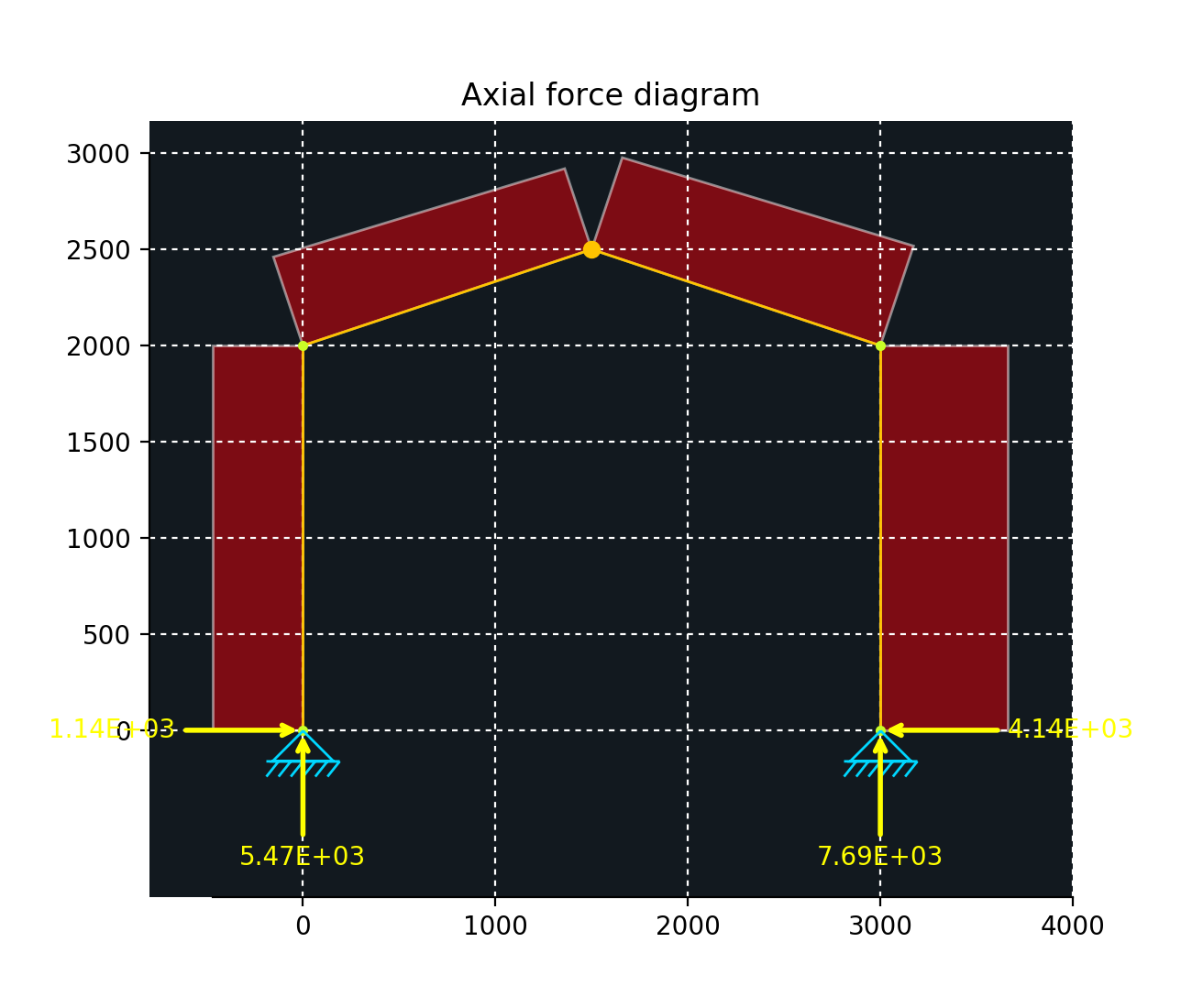
# plot the axial force along the frame elements
ax3 = disp.plot_internal_forces(ax=ax3, result=res, component='axial')
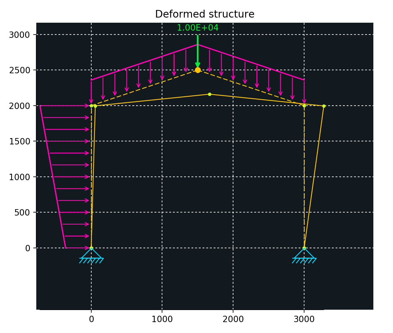
# plot the deformed shape of the structure
ax4 = disp.plot_deformed_geometry(ax=ax4, result=res, show_undeformed=True,
scale=500)

